Solve a Day Ahead Market Scheduling Problem using SIIP

In this tutorial, you will create and solve a day ahead market scheduling problem using SIIP.

Once you have completed this tutorial, you will have a basic understanding of a simple workflow in Julia when using packages under the SIIP umbrella.

If you are already familiar with this or want to jump ahead, you may want to check out the tutorial on manipulating data in PowerSystems.System.

Setup

If you haven't done so already, you will need to set up your local development environment.

Create a entry point script file

Using vscode, you can create a new file anywhere in this folder.

I personally like to make all my scripts a Julia package. For creating this repository, I did the following:

(@v1.9) pkg> generate SIIP_Tutorial

Then I ran the following:

cd SIIP_Tutorial
julia --project

julia --project="/path/to/any/julia-environment-folder/"

If I were starting a fresh project for an analysis, I would run generate AnalysisProjectFoo and then place my scripts in ./scripts/script-name.jl, and run using AnalysisProjectFoo in the first line. This way, I can place the functions I'm using in the package, i.e. in src/AnalysisProjectFoo.jl and write very simple function calls in ./scripts/script-name.jl.

But for this tutorial, we are not going to worry about that. You can create a entry point script file anywhere in this folder. I've created a placeholder file in ./scripts/unit-commitment.jl for this tutorial that you may use if you'd like.

SIIP is a collection of packages written in Julia that enable among other things production cost modeling. Any file that has the extension .jl is a Julia file.

In order to run this file, we will use a vscode's feature. First type println("hello world") in the unit-commitment.jl file.

Open the command palette:

• Ctrl + Shift + P on Windows
• Cmd + Shift + P on Mac

And type "Julia execute active file" and hit enter. You should see a terminal with a Julia REPL open up in the bottom half of your screen with the words hello world printed.

Verify Project Environment

We will go over environments in more detail in a next tutorial. For now, it is sufficient to know that if you cloned the repo and opened the Julia REPL from within the git repository's root directly, you are currently in a Julia environment set up for this tutorial.

To verify this, type ] in the Julia REPL to enter the REPL's Pkg (Package) mode, and type status.

If the Pkg mode prompts you to instantiate, type instantiate and hit enter. This may take a few minutes while it precompiles all the packages on your machine locally.

To exit the Pkg REPL mode, hit Backspace. You'll return back to a Julia REPL.

Type the following in the REPL to ensure that your environment is loaded correctly.

using PowerSystems

Loading PowerSystems Data

A good way to think about Production Cost Modeling is in 3 steps.

1. Loading input data into memory
2. Building a optimization problem that you'd like to solve:
   • What is the objective function?
   • What are the constraints?
3. Running the built optimization problem using the data loaded
4. Storing / visualizing results

Let's start with loading data.

For now, we are going to use an existing data set to get started but in a later tutorial, we'll walk through how to bring your own data set into a PCM with SIIP.

In your file, add the following:

using PowerSystems
using PowerSystemCaseBuilder

# uses RTS Test System with Time Series data
@time system = build_system(PSITestSystems, "modified_RTS_GMLC_DA_sys"; force_build = true, skip_serialization = true)

The code above builds a system using the modified_RTS_GMLC_DA_sys test system from the library of cases.

Once you have added the code to your file, run the file using the Julia: Execute active file in REPL command palette option.

Vscode also has a button at the top right that you can click to execute the active file in the REPL, but I like using the command palette option because it is more flexible and more general purpose. Any functionality available in vscode can be accessed using the command palette.

The Julia extension also has a feature that lets you run the current line in the REPL using Ctrl + Enter. You can also run the visually selected lines in the REPL, although there may not be a key mapping for that by default.

Once the build_system function is completed, you should see a summary of the system loaded in the Julia REPL like so.

using Logging
@info "Building the RTS test system"

using PowerSystems
using PowerSystemCaseBuilder

# uses RTS Test System with Time Series data
@time system = build_system(PSITestSystems, "modified_RTS_GMLC_DA_sys"; force_build = true, skip_serialization = true)

[ Info: Building the RTS test system

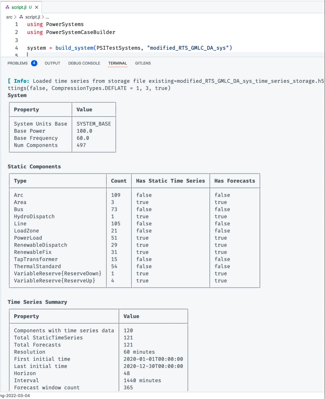
Going forward in this tutorial, I'm going to show the output of the terminal on this webpage, instead of screenshots of the vscode terminal, for the clarity of presentation. For example, the output of the system will be as follows:

  1.900906 seconds (8.94 M allocations: 450.199 MiB, 5.79% gc time, 23.47% compilation time)
System
┌───────────────────┬─────────────┐
│ Property          │ Value       │
├───────────────────┼─────────────┤
│ System Units Base │ SYSTEM_BASE │
│ Base Power        │ 100.0       │
│ Base Frequency    │ 60.0        │
│ Num Components    │ 500         │
└───────────────────┴─────────────┘

Static Components
┌───────────────────────────────────────────┬───────┬────────────────────────┬───────────────┐
│ Type                                      │ Count │ Has Static Time Series │ Has Forecasts │
├───────────────────────────────────────────┼───────┼────────────────────────┼───────────────┤
│ Arc                                       │ 109   │ false                  │ false         │
│ Area                                      │ 3     │ true                   │ true          │
│ Bus                                       │ 73    │ false                  │ false         │
│ FixedAdmittance                           │ 3     │ true                   │ true          │
│ HydroDispatch                             │ 1     │ true                   │ true          │
│ Line                                      │ 105   │ false                  │ false         │
│ LoadZone                                  │ 21    │ false                  │ false         │
│ PowerLoad                                 │ 51    │ true                   │ true          │
│ RenewableDispatch                         │ 29    │ true                   │ true          │
│ RenewableFix                              │ 31    │ true                   │ true          │
│ TapTransformer                            │ 15    │ false                  │ false         │
│ ThermalStandard                           │ 54    │ false                  │ false         │
│ VariableReserve{PowerSystems.ReserveDown} │ 1     │ true                   │ true          │
│ VariableReserve{PowerSystems.ReserveUp}   │ 4     │ true                   │ true          │
└───────────────────────────────────────────┴───────┴────────────────────────┴───────────────┘

Time Series Summary
┌──────────────────────────────────┬─────────────────────┐
│ Property                         │ Value               │
├──────────────────────────────────┼─────────────────────┤
│ Components with time series data │ 123                 │
│ Total StaticTimeSeries           │ 124                 │
│ Total Forecasts                  │ 124                 │
│ Resolution                       │ 60 minutes          │
│ First initial time               │ 2020-01-01T00:00:00 │
│ Last initial time                │ 2020-12-30T00:00:00 │
│ Horizon                          │ 48                  │
│ Interval                         │ 1440 minutes        │
│ Forecast window count            │ 365                 │
└──────────────────────────────────┴─────────────────────┘

The summary shows us that this system has 3 areas, 73 buses, and a mix of renewable and thermal generation.

@time system = build_system(PSITestSystems, "modified_RTS_GMLC_DA_sys";
   force_build = true, skip_serialization = true);
@time system = build_system(PSITestSystems, "modified_RTS_GMLC_DA_sys";
   force_build = true, skip_serialization = true);
@time system = build_system(PSITestSystems, "modified_RTS_GMLC_DA_sys";
   force_build = true, skip_serialization = true);

  1.491860 seconds (8.49 M allocations: 425.314 MiB, 7.42% gc time)
  1.498066 seconds (8.49 M allocations: 425.314 MiB, 12.36% gc time)
  1.392384 seconds (8.49 M allocations: 425.381 MiB, 4.70% gc time)

Also, notice that we ran the function build_system and stored the returned value in a variable called system. We can see the type of any value by calling the typeof function. You can type the following in the Julia REPL.

typeof(system)

PowerSystems.System

This is a PowerSystems.System type. Here PowerSystems is the Julia Module i.e. Package where the type is defined. System is the type.

This PowerSystems.System struct contains all the data for our 73 bus test system.

typeof(system);

typeof(system)
nothing

PowerSystemCaseBuilder comes with a large number of other test systems.

using PowerSystemCaseBuilder
show_categories()

PowerSystemCaseBuilder.MatPowerTestSystems
PowerSystemCaseBuilder.PSITestSystems
PowerSystemCaseBuilder.PSSETestSystems
PowerSystemCaseBuilder.PSYTestSystems
PowerSystemCaseBuilder.SIIPExampleSystems

We will discuss more about these other systems, and how this data can be accessed or modified in a later part of this tutorial.

Building a Optimization Problem

Let's solve a day ahead unit commitment problem. First, we need to define the list of constraints that define a unit commitment problem. Fortunately, PowerSimulations has a template for just that.

using PowerSimulations

@info "Building a template for unit commitment"
template = template_unit_commitment()

Network Model
┌───────────────┬────────────────────────────────────────┐
│ Network Model │ PowerSimulations.CopperPlatePowerModel │
│ Slacks        │ false                                  │
│ PTDF          │ false                                  │
│ Duals         │                                        │
└───────────────┴────────────────────────────────────────┘

Device Models
┌───────────────────────────────────┬─────────────────────────────────────────────┬────────┐
│ Device Type                       │ Formulation                                 │ Slacks │
├───────────────────────────────────┼─────────────────────────────────────────────┼────────┤
│ PowerSystems.ThermalStandard      │ PowerSimulations.ThermalBasicUnitCommitment │ false  │
│ PowerSystems.HydroEnergyReservoir │ PowerSimulations.HydroDispatchRunOfRiver    │ false  │
│ PowerSystems.RenewableDispatch    │ PowerSimulations.RenewableFullDispatch      │ false  │
│ PowerSystems.PowerLoad            │ PowerSimulations.StaticPowerLoad            │ false  │
│ PowerSystems.InterruptibleLoad    │ PowerSimulations.InterruptiblePowerLoad     │ false  │
│ PowerSystems.RenewableFix         │ PowerSimulations.FixedOutput                │ false  │
│ PowerSystems.HydroDispatch        │ PowerSimulations.HydroDispatchRunOfRiver    │ false  │
└───────────────────────────────────┴─────────────────────────────────────────────┴────────┘

Branch Models
┌─────────────────────────────┬───────────────────────────────┬────────┐
│ Branch Type                 │ Formulation                   │ Slacks │
├─────────────────────────────┼───────────────────────────────┼────────┤
│ PowerSystems.Transformer2W  │ PowerSimulations.StaticBranch │ false  │
│ PowerSystems.Line           │ PowerSimulations.StaticBranch │ false  │
│ PowerSystems.HVDCLine       │ PowerSimulations.HVDCDispatch │ false  │
│ PowerSystems.TapTransformer │ PowerSimulations.StaticBranch │ false  │
└─────────────────────────────┴───────────────────────────────┴────────┘

Service Models
┌────────────────────────────────────────────────────────┬───────────────────────────────┬────────┬──────────────────┐
│ Service Type                                           │ Formulation                   │ Slacks │ Aggregated Model │
├────────────────────────────────────────────────────────┼───────────────────────────────┼────────┼──────────────────┤
│ PowerSystems.VariableReserve{PowerSystems.ReserveUp}   │ PowerSimulations.RangeReserve │ false  │ true             │
│ PowerSystems.VariableReserve{PowerSystems.ReserveDown} │ PowerSimulations.RangeReserve │ false  │ true             │
└────────────────────────────────────────────────────────┴───────────────────────────────┴────────┴──────────────────┘

This template is like a blueprint or recipe for what optimization problem we'd like to solve.

Note that this printout shows that this template defines the recipe for how to assemble device, branch and service models. And under device models, for the various kinds of components, there are various formulations assigned to them. All of this is configurable, but for now we are going to stick with the defaults. We will discuss the various kinds of device formulations in a later tutorial.

Next, we want to choose a solver that can solve mixed integer linear programming (MILP) problems. GLPK, Cbc, Gurobi, CPLEX, Xpress etc are all valid options here. For this tutorial we are going to use HiGHS.

using HiGHS

optimizer = optimizer_with_attributes(HiGHS.Optimizer, "mip_rel_gap" => 0.05)

MathOptInterface.OptimizerWithAttributes(HiGHS.Optimizer, Pair{MathOptInterface.AbstractOptimizerAttribute, Any}[MathOptInterface.RawOptimizerAttribute("mip_rel_gap") => 0.05])

Note that the pair "mip_rel_gap" => 0.05 argument passed to this function is a solver option of HiGHS. If you are using a different solver, you may need to look up the options in the solver interface in the corresponding Julia package. For example, if you wanted to use Cbc, you could replace HiGHS.Optimizer with Cbc.Optimizer and add the corresponding attributes for the Cbc solver. For more information on this, check out the JuMP documentation.

In order to build a model, we can create an instance of a DecisionModel using the template that defines the optimization problem and the system that contains the input data. We also pass in additional options for the optimizer and the horizon in this case.

model = DecisionModel(
   template,
   system;
   optimizer = optimizer,
   horizon = 24,
)
build!(model, output_dir = mktempdir())

PowerSimulations.BuildStatusModule.BuildStatus.BUILT = 0

Note that the build! function uses the data in the system to assemble the optimization model (create all the variables, constraints, objective function etc, defined in the template) that we can pass to the solver.

Solving the Optimization Model

The build! function is where most of the heavy lifting is done. Now that the model is built, we can solve the model by calling solve!.

solve!(model)

This sends the JuMP model to the solver, in our case HiGHS, and solves an optimization problem. When this successfully completes, you should see the following status message being printed out to your terminal.

PowerSimulations.RunStatusModule.RunStatus.SUCCESSFUL = 0

Getting Results from the Model

Now that we've built and solved the model, we can get results from it.

PowerSimulations has some helper functionality to this end.

results = ProblemResults(model)

Start: 2020-01-01T00:00:00
End: 2020-01-01T23:00:00
Resolution: 60 minutes

PowerSimulations Problem Auxiliary variables Results
┌─────────────────────────────┐
│ EnergyOutput__HydroDispatch │
└─────────────────────────────┘

PowerSimulations Problem Expressions Results
┌─────────────────────────────────────────────┐
│ ProductionCostExpression__ThermalStandard   │
│ ProductionCostExpression__HydroDispatch     │
│ ProductionCostExpression__RenewableDispatch │
└─────────────────────────────────────────────┘

PowerSimulations Problem Parameters Results
┌─────────────────────────────────────────────────────────────────────────────────────┐
│ RequirementTimeSeriesParameter__VariableReserve__PowerSystems.ReserveUp__Spin_Up_R1 │
│ RequirementTimeSeriesParameter__VariableReserve__PowerSystems.ReserveUp__Spin_Up_R3 │
│ ActivePowerTimeSeriesParameter__RenewableDispatch                                   │
│ ActivePowerTimeSeriesParameter__RenewableFix                                        │
│ ActivePowerTimeSeriesParameter__HydroDispatch                                       │
│ RequirementTimeSeriesParameter__VariableReserve__PowerSystems.ReserveUp__Spin_Up_R2 │
│ RequirementTimeSeriesParameter__VariableReserve__PowerSystems.ReserveDown__Reg_Down │
│ ActivePowerTimeSeriesParameter__PowerLoad                                           │
│ RequirementTimeSeriesParameter__VariableReserve__PowerSystems.ReserveUp__Reg_Up     │
└─────────────────────────────────────────────────────────────────────────────────────┘

PowerSimulations Problem Variables Results
┌─────────────────────────────────────────────────────────────────────────────────┐
│ ActivePowerReserveVariable__VariableReserve__PowerSystems.ReserveUp__Spin_Up_R1 │
│ ActivePowerReserveVariable__VariableReserve__PowerSystems.ReserveUp__Spin_Up_R3 │
│ StartVariable__ThermalStandard                                                  │
│ ActivePowerVariable__ThermalStandard                                            │
│ ActivePowerVariable__RenewableDispatch                                          │
│ OnVariable__ThermalStandard                                                     │
│ ActivePowerReserveVariable__VariableReserve__PowerSystems.ReserveUp__Reg_Up     │
│ ActivePowerReserveVariable__VariableReserve__PowerSystems.ReserveUp__Spin_Up_R2 │
│ ActivePowerReserveVariable__VariableReserve__PowerSystems.ReserveDown__Reg_Down │
│ StopVariable__ThermalStandard                                                   │
│ ActivePowerVariable__HydroDispatch                                              │
└─────────────────────────────────────────────────────────────────────────────────┘

For example, if you are interested in getting the objection function value, you can use the get_objective_value function:

get_objective_value(results)

1.494376408647729e6

There are a lot of other helper functions available to get results from the model. In order to find what functions are available on to call, you can refer to the API reference documentation of PowerSimulations. Searching for res::ProblemResults on this page can help you find a method that you are interested in.

for method in methodswith(ProblemResults)
   println(method)
end

Plotting Results

In addition to getting results as values, we would also like to visualize the results. The PowerGraphics package gets data from a ProblemResults instance and visualizes it using the Plots package.

Try running the following code in your REPL:

using PowerGraphics

p = plot_fuel(results)

using Plots

plotlyjs()

using PowerGraphics

p = plot_fuel(results)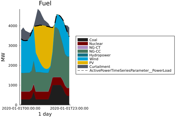

Summary

At the end of this tutorial, you should have a file that look something like this:

using Logging

@info "Building the RTS test system"
using PowerSystems
using PowerSystemCaseBuilder

# uses RTS Test System with Time Series data
system = build_system(PSITestSystems, "modified_RTS_GMLC_DA_sys"; force_build = true, skip_serialization = true)

@info "Building a template for unit commitment"
using PowerSimulations

template = template_unit_commitment()

@info "Creating a solver"
using HiGHS

optimizer = optimizer_with_attributes(HiGHS.Optimizer, "mip_rel_gap" => 0.05)

@info "Create a model"
model = DecisionModel(
   template,
   system;
   optimizer = optimizer,
   horizon = 24,
)

@info "Build the model"
build!(model, output_dir = mktempdir())

@info "Solve the model"
solve!(model)

@info "Get results"
results = ProblemResults(model)

using PowerGraphics

p = plot_fuel(results)

In this basic tutorial, we created a system using PowerSystemCaseBuilder, created the default unit commitment template, built and solved a model using an optimization solver for a 24 hours horizon, and plotted some results.

In the next tutorial, we will cover how to manipulate the input data, how to customize the formulation template and more.

Before we end, let's refactor our code in preparation for the next session. We will do 2 things:

1. Move all imports to the top of the file
2. Create functions for individual steps

using Logging

using HiGHS
using PowerGraphics
using PowerSimulations
using PowerSystemCaseBuilder
using PowerSystems


function get_system()
   @info "Building the RTS test system"
   # uses RTS Test System with Time Series data
   build_system(PSITestSystems, "modified_RTS_GMLC_DA_sys"; force_build = true, skip_serialization = true)
end


function get_template()
   @info "Building a template for unit commitment"
   template_unit_commitment()
end


function get_optimizer()
   @info "Creating a solver"
   optimizer_with_attributes(HiGHS.Optimizer, "mip_rel_gap" => 0.05)
end


function get_unit_commitment_model()
   system = get_system()
   template = get_template()
   optimizer = get_optimizer()

   @info "Create a model"
   model = DecisionModel(
      template,
      system;
      optimizer = optimizer,
      horizon = 24,
   )

   build!(model, output_dir = mktempdir())
   model
end


function plot_results(model)
   r = ProblemResults(model)
   plot_fuel(r)
end


function main()
   @info "Build the model"
   model = get_unit_commitment_model()
   @info "Solve the model"
   solve!(model)
   @info "Get results"
   plot_results(model)
end

main()

One advantage of functions is that it makes our code reusable. Another advantage is that it plays well with a Julia package called Revise. For our current workflow however, we won't need to deal with Revise just yet.